Methods for solving certain systems of linear algebraic equations. Systems of linear equations: basic concepts. A visual method for solving systems
Matrix method solutions of linear systems algebraic equations- derivation of the formula.
Let for the matrix BUT order n on the n there is an inverse matrix . Multiply both sides of the matrix equation on the left by (matrix orders A⋅X and AT allow to perform such an operation, see the article operations on matrices, properties of operations). We have ![]() . Since the operation of multiplying matrices of suitable orders is characterized by the associativity property, the last equality can be rewritten as
. Since the operation of multiplying matrices of suitable orders is characterized by the associativity property, the last equality can be rewritten as ![]() , and by definition inverse matrix (E is the identity matrix of order n on the n), That's why
, and by definition inverse matrix (E is the identity matrix of order n on the n), That's why 
Thus, the solution of a system of linear algebraic equations by the matrix method is determined by the formula. In other words, the SLAE solution is found using the inverse matrix .
We know that a square matrix BUT order n on the n has an inverse matrix only if its determinant is non-zero. Therefore, the SYSTEM n LINEAR ALGEBRAIC EQUATIONS WITH n UNKNOWN CAN BE SOLVED BY THE MATRIX METHOD ONLY WHEN THE DETERMINANT OF THE BASIC MATRIX OF THE SYSTEM IS NON-ZERO.
Top of page
Examples of solving systems of linear algebraic equations by the matrix method.
Consider the matrix method with examples. In some examples, we will not describe in detail the process of calculating the determinants of matrices, if necessary, refer to the article calculating the determinant of a matrix.
Example.
Use the inverse matrix to find the solution to the system linear equations  .
.
Decision.
In matrix form, the original system can be written as , where  . Let's calculate the determinant of the main matrix and make sure that it is different from zero. Otherwise, we will not be able to solve the system by the matrix method. We have
  , therefore, for the matrix BUT the inverse matrix can be found. Thus, if we find the inverse matrix, then the desired solution of the SLAE will be defined as . So, the task was reduced to the construction of the inverse matrix . Let's find her.
We know that for the matrix  the inverse matrix can be found as
  , where are the algebraic complements of the elements .
In our case 
Then 
Let's check the obtained solution  , substituting it into the matrix form of the original system of equations . This equality must turn into an identity, otherwise a mistake was made somewhere.
Therefore, the solution is correct.
Answer:
or in another entry ![]() .
.
Example.
Solve SLAE by matrix method.
Decision.
The first equation of the system does not contain an unknown variable x2, the second - x 1, third - x 3. That is, the coefficients in front of these unknown variables are equal to zero. We rewrite the system of equations as  . From this form it is easier to switch to the matrix form of the SLAE notation
  . Let us make sure that this system of equations can be solved using the inverse matrix. In other words, we will show that:
Let's build an inverse matrix using a matrix of algebraic additions: 
then, 
It remains to find the solution to the SLAE: 
Answer:
 .
.
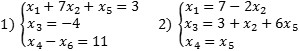
When passing from the usual form of a system of linear algebraic equations to its matrix form, one should be careful with the order of the unknown variables in the equations of the system. For example, SLAU  CANNOT be written as
  . You must first order all unknown variables in all equations of the system, and then proceed to matrix notation:
or 
Also, be careful with the notation of unknown variables, instead of x 1 , x 2 , …, x n can be any other letters. For example, SLAU  in matrix form is written as
  .
.
Let's take an example.
Example.
 using an inverse matrix.
Decision.
Having ordered the unknown variables in the equations of the system, we write it in the matrix form  . Calculate the determinant of the main matrix:
It is non-zero, so the solution to the system of equations can be found using the inverse matrix as  . Find the inverse matrix by the formula
  :
:
We get the desired solution: 
Answer:
x=0, y=-2, z=3.
Example.
Find a solution to a system of linear algebraic equations  matrix method.
Decision.
The determinant of the main matrix of the system is equal to zero 
therefore, we cannot apply the matrix method.
Finding a solution to such systems is described in the section on solving systems of linear algebraic equations.
Example.
Solve SLAE  matrix method, is some real number.
Decision.
The system of equations in matrix form has the form  . Let's calculate the determinant of the main matrix of the system and make sure that it is different from zero:
The square trinomial does not vanish for any actual values, since its discriminant is negative, so the determinant of the main matrix of the system is not equal to zero for any real . By the matrix method, we have  . Let's construct the inverse matrix by the formula :
Then 
Answer:
 .Back to top
Summarize.
The matrix method is suitable for solving SLAEs in which the number of equations coincides with the number of unknown variables and the determinant of the main matrix of the system is nonzero. If the system contains more than three equations, then finding the inverse matrix requires significant computational effort, therefore, in this case, it is advisable to use the Gauss method for solving.
Example 1. To find common decision and some particular solution of the systemDecision do it with a calculator. We write out the extended and main matrices: 
The dotted line separates the main matrix A. We write the unknown systems from above, bearing in mind the possible permutation of the terms in the equations of the system. Determining the rank of the extended matrix, we simultaneously find the rank of the main one. In matrix B, the first and second columns are proportional. Of the two proportional columns, only one can fall into the basic minor, so let's move, for example, the first column beyond the dashed line with the opposite sign. For the system, this means the transfer of terms from x 1 to the right side of the equations. 
We bring the matrix to a triangular form. We will work only with rows, since multiplying a row of a matrix by a non-zero number and adding it to another row for the system means multiplying the equation by the same number and adding it to another equation, which does not change the solution of the system. Working with the first row: multiply the first row of the matrix by (-3) and add to the second and third rows in turn. Then we multiply the first row by (-2) and add it to the fourth one. 
The second and third lines are proportional, therefore, one of them, for example the second, can be crossed out. This is equivalent to deleting the second equation of the system, since it is a consequence of the third one. 
Now we work with the second line: multiply it by (-1) and add it to the third. 
The dashed minor has the highest order (of the possible minors) and is non-zero (it is equal to the product elements on the main diagonal), and this minor belongs to both the main matrix and the extended one, hence rangA = rangB = 3 .
Minor  is basic. It includes coefficients for unknown x 2, x 3, x 4, which means that the unknown x 2, x 3, x 4 are dependent, and x 1, x 5 are free.
We transform the matrix, leaving only the basic minor on the left (which corresponds to point 4 of the above solution algorithm). 
The system with coefficients of this matrix is equivalent to the original system and has the form

x 4 =3-4x 5 , x 3 =3-4x 5 -2x 4 =3-4x 5 -6+8x 5 =-3+4x 5
x 2 =x 3 +2x 4 -2+2x 1 +3x 5 = -3+4x 5 +6-8x 5 -2+2x 1 +3x 5 = 1+2x 1 -x 5
We got relations expressing dependent variables x 2, x 3, x 4 through free x 1 and x 5, that is, we found a general solution:

Giving arbitrary values to the free unknowns, we obtain any number of particular solutions. Let's find two particular solutions:
1) let x 1 = x 5 = 0, then x 2 = 1, x 3 = -3, x 4 = 3;
2) put x 1 = 1, x 5 = -1, then x 2 = 4, x 3 = -7, x 4 = 7.
Thus, we found two solutions: (0.1, -3,3,0) - one solution, (1.4, -7.7, -1) - another solution.
Example 2. Investigate compatibility, find a general and one particular solution of the system 
Decision. Let's rearrange the first and second equations to have a unit in the first equation and write the matrix B. 
We get zeros in the fourth column, operating on the first row: 
Now get the zeros in the third column using the second row: 
 The third and fourth rows are proportional, so one of them can be crossed out without changing the rank:
Multiply the third row by (-2) and add to the fourth: 
We see that the ranks of the main and extended matrices are 4, and the rank coincides with the number of unknowns, therefore, the system has a unique solution:
-x 1 \u003d -3 → x 1 \u003d 3; x 2 \u003d 3-x 1 → x 2 \u003d 0; x 3 \u003d 1-2x 1 → x 3 \u003d 5.
x 4 \u003d 10- 3x 1 - 3x 2 - 2x 3 \u003d 11.
Example 3. Examine the system for compatibility and find a solution if it exists. 
Decision. We compose the extended matrix of the system. 
 Rearrange the first two equations so that there is a 1 in the upper left corner:
Multiplying the first row by (-1), we add it to the third: 
Multiply the second line by (-2) and add to the third: 
The system is inconsistent, since the main matrix received a row consisting of zeros, which is crossed out when the rank is found, and the last row remains in the extended matrix, that is, r B > r A .
Exercise. Investigate this system of equations for compatibility and solve it by means of matrix calculus.
Decision
Example. Prove the compatibility of a system of linear equations and solve it in two ways: 1) by the Gauss method; 2) Cramer's method. (enter the answer in the form: x1,x2,x3)
Solution :doc :doc :xls
Answer: 2,-1,3.
Example. A system of linear equations is given. Prove its compatibility. Find a general solution of the system and one particular solution.
Decision
Answer: x 3 \u003d - 1 + x 4 + x 5; x 2 \u003d 1 - x 4; x 1 = 2 + x 4 - 3x 5
Exercise. Find general and particular solutions for each system.
Decision. We study this system using the Kronecker-Capelli theorem.
We write out the extended and main matrices:
| 1 | 1 | 14 | 0 | 2 | 0 |
| 3 | 4 | 2 | 3 | 0 | 1 |
| 2 | 3 | -3 | 3 | -2 | 1 |
| x 1 | x2 | x 3 | x4 | x5 |
Here matrix A is in bold type.
We bring the matrix to a triangular form. We will work only with rows, since multiplying a row of a matrix by a non-zero number and adding it to another row for the system means multiplying the equation by the same number and adding it to another equation, which does not change the solution of the system.
Multiply the 1st row by (3). Multiply the 2nd row by (-1). Let's add the 2nd line to the 1st:
| 0 | -1 | 40 | -3 | 6 | -1 |
| 3 | 4 | 2 | 3 | 0 | 1 |
| 2 | 3 | -3 | 3 | -2 | 1 |
Multiply the 2nd row by (2). Multiply the 3rd row by (-3). Let's add the 3rd line to the 2nd:
| 0 | -1 | 40 | -3 | 6 | -1 |
| 0 | -1 | 13 | -3 | 6 | -1 |
| 2 | 3 | -3 | 3 | -2 | 1 |
Multiply the 2nd row by (-1). Let's add the 2nd line to the 1st:
| 0 | 0 | 27 | 0 | 0 | 0 |
| 0 | -1 | 13 | -3 | 6 | -1 |
| 2 | 3 | -3 | 3 | -2 | 1 |
The selected minor has the highest order (of all possible minors) and is different from zero (it is equal to the product of the elements on the reciprocal diagonal), and this minor belongs to both the main matrix and the extended one, therefore rang(A) = rang(B) = 3 Since the rank of the main matrix is equal to the rank of the extended one, then the system is collaborative.
This minor is basic. It includes coefficients for unknown x 1, x 2, x 3, which means that the unknown x 1, x 2, x 3 are dependent (basic), and x 4, x 5 are free.
We transform the matrix, leaving only the basic minor on the left.
| 0 | 0 | 27 | 0 | 0 | 0 |
| 0 | -1 | 13 | -1 | 3 | -6 |
| 2 | 3 | -3 | 1 | -3 | 2 |
| x 1 | x2 | x 3 | x4 | x5 |
27x3=
- x 2 + 13x 3 = - 1 + 3x 4 - 6x 5
2x 1 + 3x 2 - 3x 3 = 1 - 3x 4 + 2x 5
By the method of elimination of unknowns we find:
We got relations expressing dependent variables x 1, x 2, x 3 through free x 4, x 5, that is, we found common decision:
x 3 = 0
x2 = 1 - 3x4 + 6x5
x 1 = - 1 + 3x 4 - 8x 5
uncertain, because has more than one solution.
Exercise. Solve the system of equations.
Answer:x 2 = 2 - 1.67x 3 + 0.67x 4
x 1 = 5 - 3.67x 3 + 0.67x 4
Giving arbitrary values to the free unknowns, we obtain any number of particular solutions. The system is uncertain
A system of linear equations is a union of n linear equations, each containing k variables. It is written like this:
Many, when faced with higher algebra for the first time, mistakenly believe that the number of equations must necessarily coincide with the number of variables. In school algebra this is usually the case, but for higher algebra this is, generally speaking, not true.
The solution of a system of equations is a sequence of numbers (k 1 , k 2 , ..., k n ), which is the solution to each equation of the system, i.e. when substituting into this equation instead of variables x 1 , x 2 , ..., x n gives the correct numerical equality.
Accordingly, to solve a system of equations means to find the set of all its solutions or to prove that this set is empty. Since the number of equations and the number of unknowns may not be the same, three cases are possible:
- The system is inconsistent, i.e. the set of all solutions is empty. Enough rare case, which is easily detected no matter how the system is solved.
- The system is consistent and defined, i.e. has exactly one solution. The classic version, well known since school.
- The system is consistent and undefined, i.e. has infinitely many solutions. This is the hardest option. It is not enough to state that "the system has an infinite set of solutions" - it is necessary to describe how this set is arranged.
The variable x i is called allowed if it is included in only one equation of the system, and with a coefficient of 1. In other words, in the remaining equations, the coefficient for the variable x i must be equal to zero.
If we select one allowed variable in each equation, we get a set of allowed variables for the entire system of equations. The system itself, written in this form, will also be called allowed. Generally speaking, one and the same initial system can be reduced to different allowed systems, but this does not concern us now. Here are examples of allowed systems:
Both systems are allowed with respect to the variables x 1 , x 3 and x 4 . However, with the same success it can be argued that the second system is allowed with respect to x 1 , x 3 and x 5 . It is enough to rewrite the latest equation in the form x 5 = x 4 .
Now consider a more general case. Suppose we have k variables in total, of which r are allowed. Then two cases are possible:
- The number of allowed variables r is equal to the total number of variables k : r = k . We get a system of k equations in which r = k allowed variables. Such a system is collaborative and definite, because x 1 \u003d b 1, x 2 \u003d b 2, ..., x k \u003d b k;
- The number of allowed variables r is less than total number variables k : r< k . Остальные (k − r ) переменных называются свободными - они могут принимать любые значения, из которых легко вычисляются разрешенные переменные.
So, in the above systems, the variables x 2 , x 5 , x 6 (for the first system) and x 2 , x 5 (for the second) are free. The case when there are free variables is better formulated as a theorem:
Please note: this is a very important point! Depending on how you write the final system, the same variable can be both allowed and free. Most advanced math tutors recommend writing out variables in lexicographic order, i.e. ascending index. However, you don't have to follow this advice at all.
Theorem. If in a system of n equations the variables x 1 , x 2 , ..., x r are allowed, and x r + 1 , x r + 2 , ..., x k are free, then:
- If we set the values of free variables (x r + 1 = t r + 1 , x r + 2 = t r + 2 , ..., x k = t k ), and then find the values x 1 , x 2 , ..., x r , we get one of solutions.
- If the values of the free variables in two solutions are the same, then the values of the allowed variables are also the same, i.e. solutions are equal.
What is the meaning of this theorem? To obtain all solutions of the allowed system of equations, it suffices to single out the free variables. Then, by assigning different values to free variables, we get turnkey solutions. That's all - in this way you can get all the solutions of the system. There are no other solutions.
Conclusion: the allowed system of equations is always consistent. If the number of equations in the allowed system is equal to the number of variables, the system will be definite; if less, it will be indefinite.
And everything would be fine, but the question arises: how to get the resolved one from the original system of equations? For this there is
matrix form
The system of linear equations can be represented in matrix form as:

or, according to the rule of matrix multiplication,
AX = B.If a column of free terms is added to the matrix A, then A is called the augmented matrix.
Solution Methods
Direct (or exact) methods allow you to find a solution in a certain number of steps. Iterative methods are based on the use of an iterative process and allow you to get a solution as a result of successive approximations
Direct Methods
- Sweep method (for tridiagonal matrices)
- Cholesky decomposition or method square roots(for positive-definite symmetric and Hermitian matrices)
Iterative Methods
Solving a system of linear algebraic equations in VBA
Option Explicit Sub rewenie() Dim i As Integer Dim j As Integer Dim r() As Double Dim p As Double Dim x() As Double Dim k As Integer Dim n As Integer Dim b() As Double Dim file As Integer Dim y () As Double file = FreeFile Open "C:\data.txt" For Input As file Input #file, n ReDim x(0 To n * n - 1 ) As Double ReDim y(0 To n - 1 ) As Double ReDim r(0 To n - 1 ) As Double For i = 0 To n - 1 For j = 0 To n - 1 Input #file, x(i * n + j) Next j Input #file, y(i) Next i Close #file For i = 0 To n - 1 p = x(i * n + i) For j = 1 To n - 1 x(i * n + j) = x(i * n + j) / p Next j y (i) = y(i) / p For j = i + 1 To n - 1 p = x(j * n + i) For k = i To n - 1 x(j * n + k) = x(j * n + k) - x(i * n + k) * p Next k y(j) = y(j) - y(i) * p Next j Next i " Upper triangular matrix For i = n - 1 To 0 Step -1 p = y(i) For j = i + 1 To n - 1 p = p - x(i * n + j) * r(j) Next j r(i) = p / x(i * n + i) Next i " Backtrack For i = 0 To n - 1 MsgBox r(i) Next i "end sub
see also
Links
Notes
Wikimedia Foundation. 2010 .
See what "SLAU" is in other dictionaries:
SLAU- a system of linear algebraic equations ... Dictionary of abbreviations and abbreviations
This term has other meanings, see Slough (meanings). City and unitary unit of Slough Engl. Slough Country ... Wikipedia
- (Slough) a city in the UK, part of the industrial belt surrounding Greater London, on railway London Bristol. 101.8 thousand inhabitants (1974). Mechanical engineering, electrical, electronic, automotive and chemical ... ... Great Soviet Encyclopedia
Slough- (Slough)Slough, an industrial and commercial city in Berkshire, south. England, west of London; 97,400 inhabitants (1981); light industry began to develop in the period between the world wars ... Countries of the world. Vocabulary
Slough: Slough is a city in England, in the county of Berkshire SLAU System of linear algebraic equations ... Wikipedia
Commune of Röslau Röslau Coat of arms ... Wikipedia
City of Bad Vöslau Bad Vöslau Coat of arms ... Wikipedia
Projection methods for solving SLAE are a class of iterative methods in which the problem of projecting an unknown vector onto a certain space is solved optimally with respect to some other space. Contents 1 Problem statement ... Wikipedia
City of Bad Vöslau Bad Vöslau Country AustriaAustria ... Wikipedia
The fundamental system of solutions (FSR) is a set of linearly independent solutions of a homogeneous system of equations. Content 1 Homogeneous systems 1.1 Example 2 Inhomogeneous systems ... Wikipedia
Books
- Direct and inverse problems of image reconstruction, spectroscopy and tomography with MatLab (+CD), Sizikov Valery Sergeevich. The book describes the use of the apparatus of integral equations (IU), systems of linear algebraic equations (SLAE) and systems of linear-nonlinear equations (SLNU), as well as software tools ...
